Reference sheet
Oscilloscope basics
1x vs 10x, compensation, triggering, aliasing
Oscilloscope basics
A scope shows you the probe plus the circuit, never the circuit on its own. Nearly every "weird waveform" is the measurement setup rather than the board: the wrong attenuation, an uncompensated probe, or a long ground lead ringing.
| 1× probe | 10× probe | |
|---|---|---|
| Attenuation | None — 1:1 | 10:1, so the scope sees a tenth of the signal |
| Resistance at the tip | 1 MΩ | 10 MΩ |
| Capacitance at the tip | ≈50–120 pF (the whole cable hangs on the node) | ≈9–15 pF |
| Usable bandwidth | Typically 6–20 MHz, whatever the probe body claims | The probe’s full rating — 100 MHz, 350 MHz, 500 MHz |
| Noise and smallest usable signal | Best: nothing is thrown away ahead of the input | 10× worse, because the scope’s own noise floor is now ten times larger relative to the signal |
| Use it for | Slow, small signals — millivolt sensors, audio, low-frequency ripple | Everything else. This is the default position |
On older scopes the switch on the probe body tells the instrument nothing. If the channel menu still says 1× while the probe is switched to 10×, every voltage you read is ten times too small — check that the two agree before you believe a number.
| Setting | What it does, and what it costs you |
|---|---|
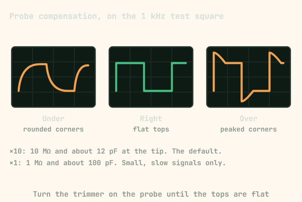
| Probe compensation | Every probe has a trimmer that matches it to this particular input, which is 15–25 pF and varies from channel to channel. Clip it to the scope’s calibration output — usually a 1 kHz square wave — and adjust for flat tops: overshooting corners mean overcompensated, rounded corners undercompensated. Redo it whenever the probe moves to another channel or another scope. An uncompensated 10× probe distorts every edge and every amplitude you measure for the rest of the day. |
| Bandwidth | The −3 dB point, not a wall: a sine right at the rated bandwidth reads about 30 % low, and it is already a few percent low at a third of it. For amplitudes you can trust, keep the highest frequency of interest below a fifth of the scope’s bandwidth. |
| Rise time | For a typical scope, tr ≈ 0.35 / bandwidth — 3.5 ns on a 100 MHz scope, 1 ns on 350 MHz. What you see is the combination: t_displayed = √(t_signal² + t_scope² + t_probe²). Show a 100 MHz scope a 2 ns edge and it draws a 4 ns one, and no setting in the menu fixes that. |
| Ground lead | The 150 mm crocodile lead is roughly 150 nH; together with the probe’s ~10 pF it forms a resonator that rings near 100 MHz. That ringing is in your measurement, not in your circuit. For any fast edge, drop the lead and use the ground spring against a ground pad millimetres from the tip. |
| Earth, and what you must never clip | The probe ground is bolted to mains earth through the scope chassis. Clipping it to a node that is not at earth potential shorts that node to earth through the probe, instantly and often destructively. To look at a switching node, a high-side gate or anything mains-referenced, use a differential probe or an isolated scope — never lift the scope’s earth pin. |
| Trigger: Auto | Sweeps anyway when no trigger arrives, so there is always a trace. Useful for finding a signal in the first place, and a liar afterwards: a flat line in Auto means either "dead circuit" or "never triggered", and it looks identical either way. |
| Trigger: Normal | Sweeps only on a real trigger and holds the previous capture otherwise. This is where you work once you know what you are looking for, and the only mode that tells the truth about a rare event. |
| Trigger: Single | Arms once, captures the first event, stops. The mode for a power-up glitch, a one-shot pulse, or the fault that will not reproduce twice. |
| Trigger level, slope and holdoff | Put the level inside the real signal, not at 0 V. If the display flickers between two otherwise stable pictures, the waveform crosses that level more than once per period — raise holdoff past the repeating pattern, or trigger on pulse width instead of an edge. |
| Coupling | DC shows the true level. AC inserts a high-pass around 5–10 Hz, which is ideal for finding 20 mV of ripple riding on a 12 V rail and misleading on anything slow: a 50 Hz square wave comes back visibly sagging that was never sagging. |
| Sample rate and aliasing | Two samples per cycle only avoids aliasing in theory; you want five to ten before the shape is readable. Undersampled, a fast signal reappears as a slow drifting one that looks entirely plausible. The test is to change the timebase — a real signal keeps its frequency, an alias changes it. |
| Vertical scale and resolution | Most scopes digitise to 8 bits across the full screen height, about 256 steps in total. A trace using a quarter of the screen is using a quarter of them, so ripple measured on a small trace is mostly quantisation. Fill the screen first, then measure. |