Calculadora online gratuita

Impedância controlada

Abrir a calculadora

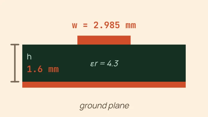
Microstrip

Exemplo w = 2.99 mm (117.5 mil) for 50 Ω on h = 1.6 mm, εr = 4.3, 0.035 mm copper.

A trace over a single reference plane, solved backwards from IPC-2141's own closed-form approximation: $Z_0=\frac{87}{\sqrt{\epsilon +1.41}}·\ln \left(\frac{5.98h}{0.8w+t}\right)$. Good to a few percent for 0.1 ≤ w/h ≤ 2 — the zone most single-ended controlled-impedance traces actually fall in.

Coplanar (CPW)

Exemplo w = 3.10 mm (122.0 mil) for 50 Ω with a 0.3 mm gap, h = 1.6 mm, εr = 4.3 — assuming no ground plane beneath this layer.

A signal trace with coplanar ground pours either side of it on the SAME layer, over a dielectric with NO continuous ground plane assumed underneath it: $Z_0=\frac{30\pi }{\sqrt{{\epsilon }_{\mathrm{eff}}}}·\frac{K\prime \left(k\right)}{K\left(k\right)}$, k = w/(w+2·gap). A ground plane close beneath (the common case on a real multilayer stack-up) needs a different, grounded-CPW formula this tool deliberately does not attempt — the published sources for it disagree with each other and could not be reconciled with confidence. Use this mode only when the layer really has no plane directly under it.

Differential pair

Exemplo w = 1.05 mm (41.4 mil) each, single-ended Z₀ = 87.07 Ω, for 100 Ω differential with a 0.2 mm gap on h = 1.6 mm, εr = 4.3.

Two matched microstrip traces, close enough to couple: $Z_{\mathrm{diff}}=2Z_0(1-0.48e^{-0.96s/h})$, where s is the EDGE-TO-EDGE gap between them and Z₀ is the single-ended impedance the same two traces would have on their own. Solved backwards from a target Zdiff — pick the gap the layout can actually hold, and this returns the width that reaches it.